概率统计学 练习题1 答案.pdf 9页

'QuantitativeMethods(M)Tutorial1ANSWERSTutorialQuestion1FundamentalstatisticalconceptsPopulationApopulationconsistsofalltheitemsthatthestatistician/researcherisinterestedin.Itmaybefiniteoreffectivelyinfinite.SampleAsampleisasubsetofitemsselectedfromthepopulationofinterest.ParameterAparameterisameasurementorcharacteristicofthepopulation.Veryoftentheparametersofapopulationareunknownbecausetheentirepopulationcannotbeobserved.StatisticAstatisticisameasureorcharacteristicdeterminedfromasample.Statisticsobtainedfromsamplesareusedtoprovideestimatesofpopulationparametersviaaprocessofstatisticalinference.DescriptivestatisticsReferstothecollection,presentationandsummaryofdatausinggraphs,tablesandnumericalmeasures.InferentialstatisticsReferstotheprocessofestimatingpopulationparameters,drawingconclusionsandmakingdecisionsaboutpopulationsonthebasisofgeneralisingfromsampleresults.(a)Thestatisticspresentedconsistofthe10%to60%rangeforthepercentageofsurveyrespondentswhoanswered‘yes’andthe45%ofUKrespondentswhoanswered‘yes’.ThesemeasuresarestatisticsbecausetheywerederivedfromthesurveyrespondentswhorepresentonlyasampleoftheentirepopulationofadultslivinginEuropeancountries.(b)Theparameterpresentedistheintervalestimateofbetween41%and49%ofadultsintheUKwhowouldbeexpectedtoanswer‘yes’.Thisrangeforthepopulationparameterhasbeenderivedfromthesamplestatisticof45%ofUKsurveyrespondentswhoanswered‘yes’.(c)Thedescriptivestatisticalanalysisthathasbeenundertakenisthedatacollectedfromthesurveyrespondentsandsubsequentlytabulatedandsummarisedbythesamplestatisticsreferredtointheanswertopart(a).(d)Theinferentialanalysisisthepredictionthatforthepopulationofall48millionadultsintheUK,thepercentagethatwouldanswer‘yes’fallsbetween41%and49%.Tutorial1Semester1,20121 QuantitativeMethods(M)TutorialQuestion2TypesofvariablesandmeasurementscalesTherearetwobasictypesofvariables:categoricalandquantitative.Categoricalvariablesarethoseforwhichthevaluesofthevariablearelabelsordescriptivewords(e.g.valuessuchasred,blue,black;small,medium,large).Quantitativevariablesarethoseforwhichthevaluesofthevariablearenumbers(e.g.incometakesonavalueof$60,000;age=26years).Quantitativevariablesaremeasuredonanintervalscale.Categoricalvariableswithorderedcategoriesaremeasuredonanordinalscale.Categoricalvariableswithunorderedcategoriesaremeasuredonanominalscale.Answers:(a)Nominal(b)Nominal(orarguablyordinal)(c)Ordinal(d)Interval(e)Interval(f)Interval(g)Ordinal(h)Interval(i)Ordinal(j)IntervalTutorialQuestion3(a)Interval(b)Ordinal(c)NominalTutorialQuestion4Answer:C1.(Thescatterplotsthatrepresentzerocorrelationare:B,D,F,H,K,M,N,PandQ.TutorialQuestion5Estimationequationis:Predictedfertility=3.2–0.04xInternetUse%Part(a)Foranationwith50%ofpeopleusingtheinternet(e.g.USA):Predictedfertility=3.2–(0.04x50)=1.2childrenperadultwoman.Foranationwith0%ofpeopleusingtheinternet(e.g.Yemen):Predictedfertility=3.2–(0.04x0)=3.2childrenperadultwoman.Tutorial1Semester1,20122 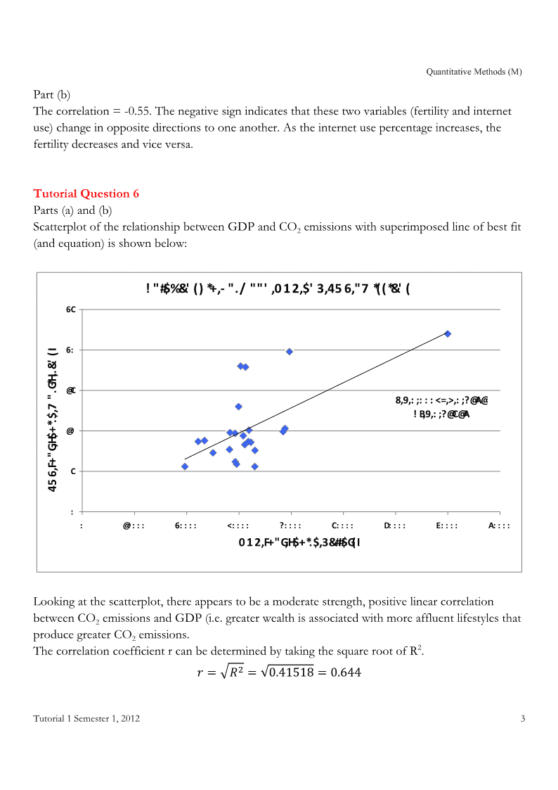QuantitativeMethods(M)Part(b)Thecorrelation=-0.55.Thenegativesignindicatesthatthesetwovariables(fertilityandinternetuse)changeinoppositedirectionstooneanother.Astheinternetusepercentageincreases,thefertilitydecreasesandviceversa.TutorialQuestion6Parts(a)and(b)ScatterplotoftherelationshipbetweenGDPandCO2emissionswithsuperimposedlineofbestfit(andequation)isshownbelow:!"#$%&"()*+,‐"./""",012,$"3,456,"7*((*&"(6C6:*H,.&"(I@C8,9,:;:::<=,>,:;?@A@!B,9,:;?@C@A.$,7".G@:,H$+*C456,F+"G::@::::6::::<::::?::::C::::D::::E::::A::::012,F+"G,H$+*.$,3&##$G(ILookingatthescatterplot,thereappearstobeamoderatestrength,positivelinearcorrelationbetweenCO2emissionsandGDP(i.e.greaterwealthisassociatedwithmoreaffluentlifestylesthatproducegreaterCO2emissions.2ThecorrelationcoefficientrcanbedeterminedbytakingthesquarerootofR.ݎൌඥܴଶൌ√0.41518ൌ0.644Tutorial1Semester1,20123 QuantitativeMethods(M)Part(c)ExcelregressionoutputobtainedusingtheDataAnalysisToolPackisshownbelow:RegressionStatisticsMultipleR0.644346499RSquare0.415182411AdjustedRSquare0.387333954StandardError3.620096164Observations23ANOVAdfSSMSFSignificanceFRegression1195.379066195.3814.908632680.000904979Residual21275.207020913.105Total22470.586087CoefficientsStandardErrortStatP-valueLower95%Upper95%Intercept0.4180702092.6899137150.15540.877973344-5.1759115746.012051992GDP0.000310978.05379E-053.86120.0009049790.0001434830.000478458Part(d)Theestimatedequation=predictedequation=fittedequationis:ܥܱଶ݁݉ଓݏݏଓ݋݊ݏ෣ൌ0.4181൅0.0003ܩܦܲNotethatthereisnoerrortermintheestimatedequation.Interpretationoftheintercept:ifGDPfelltozero,thepredictedCO2emissionswouldbe0.4181metrictons(percapita).ItwouldnotbeeconomicallymeaningfultoconsideranOECDcountryhavingaGDPequaltozero.Interpretationoftheslope:ifGDP(percapita)increasesby1dollar,thepredictedvalueofCO2emissionsincreasesby0.0003metrictons(percapita).22R(alsoknownascoefficientofdetermination)isameasureofgoodnessoffit.Here,R=0.415,whichisinterpretedas:approximately42%ofthevariationinCO2emissionsisexplainedbythevariationinGDP.Thisregressionmodeldoesnotexplaintheother58%ofvariationinthedependentvariable.Tutorial1Semester1,20124 QuantitativeMethods(M)Part(e)Theresidualplot(asproducedinExcelusingDataAnalysis>Regression)isshownbelow.ResidualPlot1050-5020000400006000080000Residuals-10GDPNotethatresidualsareobtainedbysubtractingpredictedvaluesofCO2emissionsfromthecorrespondingobserved(actual)valuesofCO2emissions.Part(f)CorrelationandcovariancematricescreatedinExcel(usingDataAnalysis)areshownbelow.CorrelationMatrixGDPCO2GDP1CO20.6443464991CovarianceMatrixGDPCO2GDP87843996.4CO227316.882820.46Tutorial1Semester1,20125 QuantitativeMethods(M)Notethatthecorrelationbetweenthevariablesinthetopmatrixisequaltothevaluethatwas2calculatedearlierbytakingthesquarerootofR.Thecorrelationcoefficientisameasureofthedegreeoflinearassociationbetweentwoquantitativevariables.Itmayalsobeconsideredasastandardizedvalueofthecovariancebetweenthevariables.Thecovarianceisameasureofthedegreetowhichthevaluesoftwovariableschangetogether.Iftheymoveinthesamedirection,thecovariancewillbepositiveandiftheymoveinoppositedirectionsthecovariancewillbenegative.Howeverthemagnitudeofthecovarianceisdifficulttointerpretbecauseitdependsontheunitsofmeasurementforthevariables.Incontrast,themagnitudeofthecorrelationcoefficientwillalwaysbebetween-1and+1.Parts(g)and(h)PredictedvaluesofCO2emissionsareobtainedbysubstitutingobservedGDPvaluesintothepredictedequation.Therewillbeapredictedvalueforeachofthe23observedvaluesofCO2.ResidualsareobtainedbysubtractingpredictedCO2valuesfromthecorrespondingobservedCO2values.TherewillbeoneresidualforeachpairofpredictedandactualvaluesofCO2emissions(23residualsintotal).TheExceloutputbelowshowsthepredictedvaluesandresidualsforeachofthe23countries.ObservationPredictedCO2Residuals19.8501134468.149886554210.45495088-1.854950876310.0880058-1.788005803410.139937867.76006214510.34237959-0.24237959169.7319446933.26805530779.529502962-3.32950296289.2194654720.58053452897.3231679661.3768320341010.69595294-3.0959529371112.49211797-2.192117974129.181216113-1.481216113139.5142654130.1857345871422.17387044-0.1738704431510.30350829-1.603508291167.6988202111.1011797891712.37612601-2.476126014186.522108213-0.922108213198.206945846-0.906945846209.604446829-3.7044468292110.69253226-5.0925322622210.00248894-0.6024889422312.756131847.043868156Tutorial1Semester1,20126 QuantitativeMethods(M)Part(i)ThegraphbelowwasproducedbyselectingthefittedplotoptionwhenrunningtheregressionanalysisinExcel’sDataAnalysis.FittedPlot252015CO21050020000400006000080000GDPCO2PredictedCO2Part(j)ThegraphbelowwasproducedbyselectingtheresidualplotoptionwhenrunningtheregressionanalysisinExcel’sDataAnalysis.ResidualPlot1050-5020000400006000080000Residuals-10GDPTutorial1Semester1,20127 QuantitativeMethods(M)Part(k)ThepredictedCO2emissionsforacountrywithapercapitaGDPof$55,000iscalculatedas:PredictedCO2=0.4181+0.0003x55,000=16.9metrictons(percapita)ThereisnocorrespondingresidualbecausetherewasnocountryobservedwithanactualGDPequalto$55,000inthedataset.Part(l)ThepredictedCO2emissionsforacountrywithapercapitaGDPof$10,000iscalculatedas:PredictedCO2=0.4181+0.0003x10,000=3.4metrictons(percapita)ThereisnocorrespondingresidualbecausetherewasnocountryobservedwithanactualGDPequalto$10,000inthedataset.Furthermore,thelowestobservedGDPvalueinthesamplewas$19,629(Portugal)soweneedtobeverycautiousaboutmakingthisout-of-samplepredictionbecauseitinvolvesextrapolatingconsiderablybelowtherangeoftheobservedGDPvalues.Part(m)Theapproximate95%confidenceintervalsarecalculatedasfollows:Intercept:0.4181േ2ݔ2.6899ൌሼെ4.962,5.798ሽSlope:0.0003േ2ݔ0.00008ൌሼ0.0001,0.0005ሽA‘loose’interpretationoftheseconfidenceintervalsisgivenbelow.Amorepreciseexplanationwillbegivenasthecourseprogresses.Weare95%confidentthatthetrueinterceptliesbetween-4.962and5.798.Asthisrangeincludeszero,wecannotruleoutthepossibilitythatthetrueinterceptiszero.Weare95%confidentthatthetrueslopeliesbetween0.0001and0.0005.Thisrangedoesnotincludezero,thereforewecanconcludethatthetrueslopeisnotzero.Part(n)Ruleofthumbassessmentofstatisticalsignificance:absolutemagnitudeoft-stat>2orequivalentlyp-value<0.05isregardedasstatisticallysignificant.Tutorial1Semester1,20128 QuantitativeMethods(M)TherelevantExcelregressionoutputisshownbelow:CoefficientsStandardErrortStatP-valueIntercept0.4180702092.6899137150.15540.877973344GDP0.000310978.05379E-053.86120.000904979Itcanbeseenthatfortheintercept,t-stat=0.1554<2andthep-value=0.878>0.05,thereforetheinterceptdoesnotsatisfytheruleofthumbandweconcludethattheinterceptisnotstatisticallysignificant.Itcanbeseenthatfortheslope(labeledastheGDPvariable),t-stat=3.861>2andthep-value=0.0009<0.05,thereforetheslopedoessatisfytheruleofthumbandweconcludethattheslopeisstatisticallysignificant.Inotherwords,thereisastatisticallysignificantassociationbetweenGDPandCO2emissions.Part(o)Weexpect/believethatthewealthofanationasmeasuredbyitsGDPwillaffectthatcountry’sCO2emissions(implyingcausationfromtheGDPtoCO2emissions)ratherthantheotherwayaround(i.e.wedon’texpectCO2emissionstoaffectthecountry’sGDP).Tutorial1Semester1,20129'