计量经济学 庞皓 第三版课后答案.docx 82页

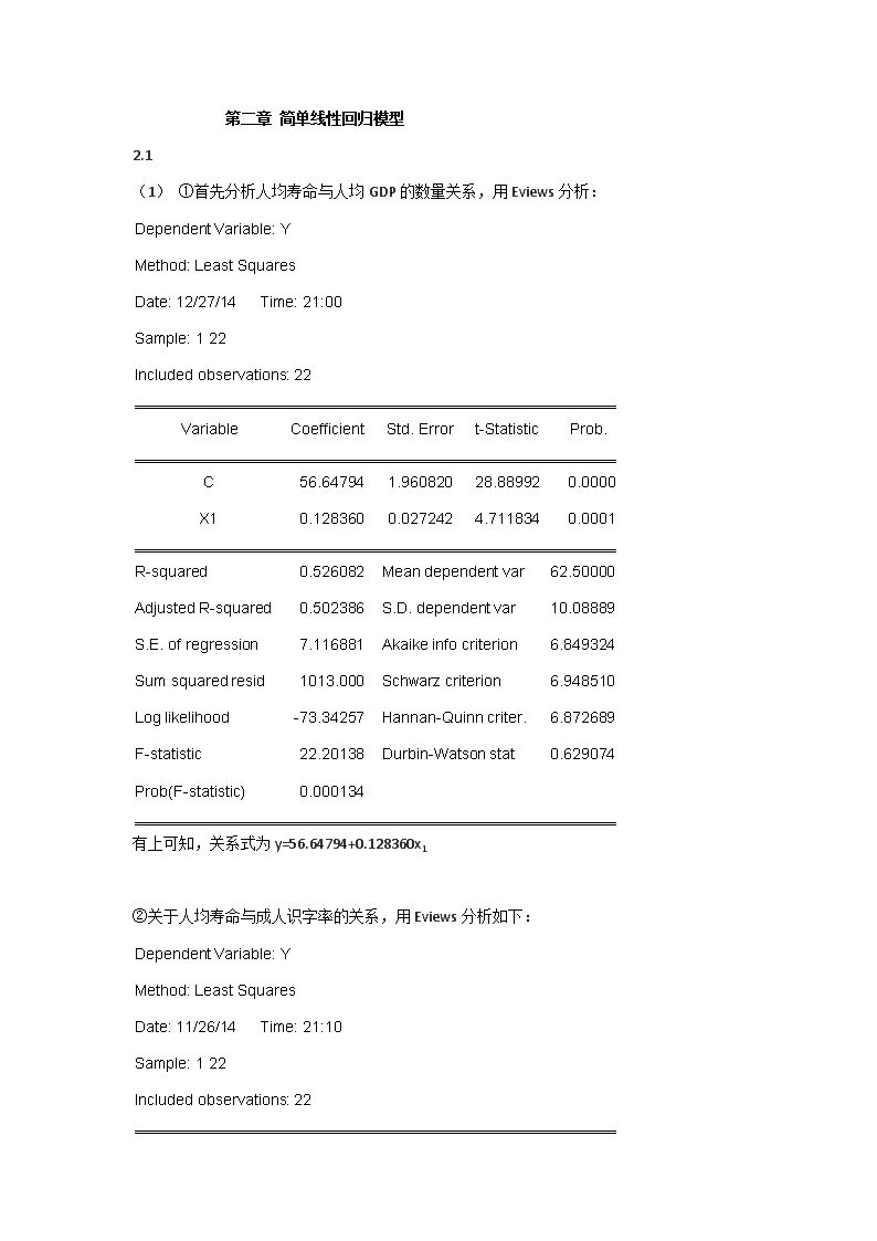
'第二章简单线性回归模型2.1（1）①首先分析人均寿命与人均GDP的数量关系，用Eviews分析：DependentVariable:YMethod:LeastSquaresDate:12/27/14Time:21:00Sample:122Includedobservations:22VariableCoefficientStd.Errort-StatisticProb.  C56.647941.96082028.889920.0000X10.1283600.0272424.7118340.0001R-squared0.526082    Meandependentvar62.50000AdjustedR-squared0.502386    S.D.dependentvar10.08889S.E.ofregression7.116881    Akaikeinfocriterion6.849324Sumsquaredresid1013.000    Schwarzcriterion6.948510Loglikelihood-73.34257    Hannan-Quinncriter.6.872689F-statistic22.20138    Durbin-Watsonstat0.629074Prob(F-statistic)0.000134有上可知，关系式为y=56.64794+0.128360x1②关于人均寿命与成人识字率的关系，用Eviews分析如下：DependentVariable:YMethod:LeastSquaresDate:11/26/14Time:21:10Sample:122Includedobservations:22 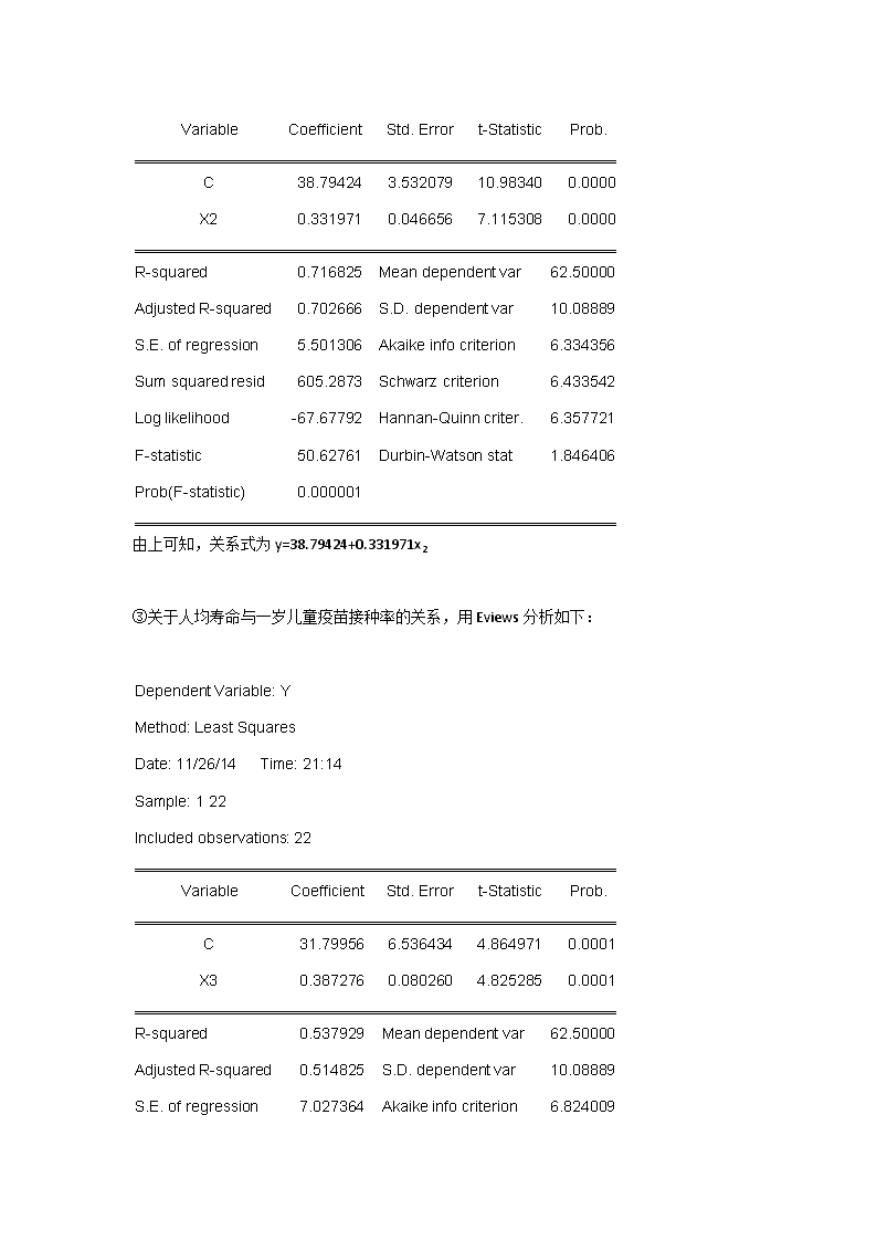VariableCoefficientStd.Errort-StatisticProb.  C38.794243.53207910.983400.0000X20.3319710.0466567.1153080.0000R-squared0.716825    Meandependentvar62.50000AdjustedR-squared0.702666    S.D.dependentvar10.08889S.E.ofregression5.501306    Akaikeinfocriterion6.334356Sumsquaredresid605.2873    Schwarzcriterion6.433542Loglikelihood-67.67792    Hannan-Quinncriter.6.357721F-statistic50.62761    Durbin-Watsonstat1.846406Prob(F-statistic)0.000001由上可知，关系式为y=38.79424+0.331971x2③关于人均寿命与一岁儿童疫苗接种率的关系，用Eviews分析如下：DependentVariable:YMethod:LeastSquaresDate:11/26/14Time:21:14Sample:122Includedobservations:22VariableCoefficientStd.Errort-StatisticProb.  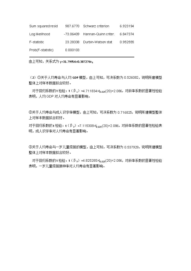C31.799566.5364344.8649710.0001X30.3872760.0802604.8252850.0001R-squared0.537929    Meandependentvar62.50000AdjustedR-squared0.514825    S.D.dependentvar10.08889S.E.ofregression7.027364    Akaikeinfocriterion6.824009 Sumsquaredresid987.6770    Schwarzcriterion6.923194Loglikelihood-73.06409    Hannan-Quinncriter.6.847374F-statistic23.28338    Durbin-Watsonstat0.952555Prob(F-statistic)0.000103由上可知，关系式为y=31.79956+0.387276x3（2）①关于人均寿命与人均GDP模型，由上可知，可决系数为0.526082，说明所建模型整体上对样本数据拟合较好。对于回归系数的t检验：t（β1）=4.711834>t0.025(20)=2.086，对斜率系数的显著性检验表明，人均GDP对人均寿命有显著影响。②关于人均寿命与成人识字率模型，由上可知，可决系数为0.716825，说明所建模型整体上对样本数据拟合较好。对于回归系数的t检验：t（β2）=7.115308>t0.025(20)=2.086，对斜率系数的显著性检验表明，成人识字率对人均寿命有显著影响。③关于人均寿命与一岁儿童疫苗的模型，由上可知，可决系数为0.537929，说明所建模型整体上对样本数据拟合较好。对于回归系数的t检验：t（β3）=4.825285>t0.025(20)=2.086，对斜率系数的显著性检验表明，一岁儿童疫苗接种率对人均寿命有显著影响。 2.2（1）①对于浙江省预算收入与全省生产总值的模型，用Eviews分析结果如下：DependentVariable:YMethod:LeastSquaresDate:12/03/14Time:17:00Sample(adjusted):133Includedobservations:33afteradjustmentsVariableCoefficientStd.Errort-StatisticProb.  X0.1761240.00407243.256390.0000C-154.306339.08196-3.9482740.0004R-squared0.983702    Meandependentvar902.5148AdjustedR-squared0.983177    S.D.dependentvar1351.009S.E.ofregression175.2325    Akaikeinfocriterion13.22880Sumsquaredresid951899.7    Schwarzcriterion13.31949Loglikelihood-216.2751    Hannan-Quinncriter.13.25931F-statistic1871.115    Durbin-Watsonstat0.100021Prob(F-statistic)0.000000②由上可知，模型的参数：斜率系数0.176124，截距为—154.3063③关于浙江省财政预算收入与全省生产总值的模型，检验模型的显著性：1）可决系数为0.983702，说明所建模型整体上对样本数据拟合较好。2）对于回归系数的t检验：t（β2）=43.25639>t0.025(31)=2.0395，对斜率系数的显著性检验表明，全省生产总值对财政预算总收入有显著影响。 ④用规范形式写出检验结果如下：Y=0.176124X—154.3063(0.004072)(39.08196)t=(43.25639)（-3.948274）R2=0.983702F=1871.115n=33⑤经济意义是：全省生产总值每增加1亿元，财政预算总收入增加0.176124亿元。（2）当x=32000时，①进行点预测，由上可知Y=0.176124X—154.3063，代入可得：Y=Y=0.176124*32000—154.3063=5481.6617②进行区间预测：先由Eviews分析：XY Mean 6000.441 902.5148 Median 2689.280 209.3900 Maximum 27722.31 4895.410 Minimum 123.7200 25.87000 Std.Dev. 7608.021 1351.009 Skewness 1.432519 1.663108 Kurtosis 4.010515 4.590432 Jarque-Bera 12.69068 18.69063 Probability 0.001755 0.000087 Sum 198014.5 29782.99  SumSq.Dev. 1.85E+09 58407195 Observations 33 33由上表可知，∑x2=∑（Xi—X）2=δ2x(n—1)= 7608.0212x(33—1)=1852223.473(Xf—X)2=(32000— 6000.441)2=675977068.2当Xf=32000时，将相关数据代入计算得到：5481.6617—2.0395x175.2325x√1/33+1852223.473/675977068.2≤Yf≤5481.6617+2.0395x175.2325x√1/33+1852223.473/675977068.2即Yf的置信区间为（5481.6617—64.9649,5481.6617+64.9649）(3)对于浙江省预算收入对数与全省生产总值对数的模型，由Eviews分析结果如下：DependentVariable:LNYMethod:LeastSquaresDate:12/03/14Time:18:00Sample(adjusted):133Includedobservations:33afteradjustmentsVariableCoefficientStd.Errort-StatisticProb.  LNX0.9802750.03429628.582680.0000C-1.9182890.268213-7.1521210.0000R-squared0.963442    Meandependentvar5.573120AdjustedR-squared0.962263    S.D.dependentvar1.684189S.E.ofregression0.327172    Akaikeinfocriterion0.662028Sumsquaredresid3.318281    Schwarzcriterion0.752726Loglikelihood-8.923468    Hannan-Quinncriter.0.692545F-statistic816.9699    Durbin-Watsonstat0.096208 Prob(F-statistic)0.000000①模型方程为：lnY=0.980275lnX-1.918289②由上可知，模型的参数：斜率系数为0.980275，截距为-1.918289③关于浙江省财政预算收入与全省生产总值的模型，检验其显著性：1）可决系数为0.963442，说明所建模型整体上对样本数据拟合较好。2）对于回归系数的t检验：t（β2）=28.58268>t0.025(31)=2.0395，对斜率系数的显著性检验表明，全省生产总值对财政预算总收入有显著影响。④经济意义：全省生产总值每增长1%，财政预算总收入增长0.980275% 2.4（1）对建筑面积与建造单位成本模型，用Eviews分析结果如下：DependentVariable:YMethod:LeastSquaresDate:12/01/14Time:12:40Sample:112Includedobservations:12VariableCoefficientStd.Errort-StatisticProb.   X-64.184004.809828-13.344340.0000C1845.47519.2644695.796880.0000R-squared0.946829    Meandependentvar1619.333AdjustedR-squared0.941512    S.D.dependentvar131.2252S.E.ofregression31.73600    Akaikeinfocriterion9.903792Sumsquaredresid10071.74    Schwarzcriterion9.984610Loglikelihood-57.42275    Hannan-Quinncriter.9.873871F-statistic178.0715    Durbin-Watsonstat1.172407Prob(F-statistic)0.000000由上可得：建筑面积与建造成本的回归方程为：Y=1845.475--64.18400X（2）经济意义：建筑面积每增加1万平方米，建筑单位成本每平方米减少64.18400元。（3）①首先进行点预测，由Y=1845.475--64.18400X得，当x=4.5，y=1556.647②再进行区间估计：用Eviews分析：YX Mean 1619.333 3.523333 Median 1630.000 3.715000 Maximum 1860.000 6.230000 Minimum 1419.000 0.600000 Std.Dev. 131.2252 1.989419 Skewness 0.003403-0.060130 Kurtosis 2.346511 1.664917  Jarque-Bera 0.213547 0.898454 Probability 0.898729 0.638121 Sum 19432.00 42.28000 SumSq.Dev. 189420.7 43.53567 Observations 12 12由上表可知，∑x2=∑（Xi—X）2=δ2x(n—1)= 1.9894192x(12—1)=43.5357(Xf—X)2=(4.5— 3.523333)2=0.95387843当Xf=4.5时，将相关数据代入计算得到：1556.647—2.228x31.73600x√1/12+43.5357/0.95387843≤Yf≤1556.647+2.228x31.73600x√1/12+43.5357/0.95387843即Yf的置信区间为（1556.647—478.1231,1556.647+478.1231） 3.1（1）①对百户拥有家用汽车量计量经济模型，用Eviews分析结果如下：DependentVariable:YMethod:LeastSquaresDate:11/25/14Time:12:38 Sample:131Includedobservations:31VariableCoefficientStd.Errort-StatisticProb.  X25.9968651.4060584.2650200.0002X3-0.5240270.179280-2.9229500.0069X4-2.2656800.518837-4.3668420.0002C246.854051.975004.7494760.0001R-squared0.666062    Meandependentvar16.77355AdjustedR-squared0.628957    S.D.dependentvar8.252535S.E.ofregression5.026889    Akaikeinfocriterion6.187394Sumsquaredresid682.2795    Schwarzcriterion6.372424Loglikelihood-91.90460    Hannan-Quinncriter.6.247709F-statistic17.95108    Durbin-Watsonstat1.147253Prob(F-statistic)0.000001②得到模型得：Y=246.8540+5.996865X2-　0.524027X3-2.265680X4③对模型进行检验：1）可决系数是0.666062，修正的可决系数为0.628957，说明模型对样本拟合较好2）F检验，F=17.95108>F（3,27）=3.65，回归方程显著。3）t检验，t统计量分别为4.749476，4.265020，-2.922950，-4.366842，均大于t（27）=2.0518，所以这些系数都是显著的。④依据：1）可决系数越大，说明拟合程度越好 1）F的值与临界值比较，若大于临界值，则否定原假设，回归方程是显著的；若小于临界值，则接受原假设，回归方程不显著。2）t的值与临界值比较，若大于临界值，则否定原假设，系数都是显著的；若小于临界值，则接受原假设，系数不显著。（2）经济意义：人均ＧＤＰ增加１万元，百户拥有家用汽车增加5.996865辆，城镇人口比重增加１个百分点，百户拥有家用汽车减少0.524027辆，交通工具消费价格指数每上升１，百户拥有家用汽车减少2.265680辆。（3）用EViews分析得：DependentVariable:YMethod:LeastSquaresDate:12/08/14Time:17:28Sample:131Includedobservations:31VariableCoefficientStd.Errort-StatisticProb.  X25.1356701.0102705.0834650.0000LNX3-22.810056.771820-3.3683780.0023LNX4-230.848149.46791-4.6666240.0001C1148.758228.29175.0319740.0000R-squared0.691952    Meandependentvar16.77355AdjustedR-squared0.657725    S.D.dependentvar8.252535S.E.ofregression4.828088    Akaikeinfocriterion6.106692Sumsquaredresid629.3818    Schwarzcriterion6.291723Loglikelihood-90.65373    Hannan-Quinncriter.6.167008F-statistic20.21624    Durbin-Watsonstat1.150090Prob(F-statistic)0.000000 模型方程为：Y=5.135670X2-22.81005LNX3-230.8481LNX4+1148.758此分析得出的可决系数为0.691952>0.666062，拟合程度得到了提高，可这样改进。3.2（１）对出口货物总额计量经济模型，用Eviews分析结果如下：：DependentVariable:YMethod:LeastSquaresDate:12/01/14Time:20:25 Sample:19942011Includedobservations:18VariableCoefficientStd.Errort-StatisticProb.  X20.1354740.01279910.584540.0000X318.853489.7761811.9285120.0729C-18231.588638.216-2.1105730.0520R-squared0.985838    Meandependentvar6619.191AdjustedR-squared0.983950    S.D.dependentvar5767.152S.E.ofregression730.6306    Akaikeinfocriterion16.17670Sumsquaredresid8007316.    Schwarzcriterion16.32510Loglikelihood-142.5903    Hannan-Quinncriter.16.19717F-statistic522.0976    Durbin-Watsonstat1.173432Prob(F-statistic)0.000000①由上可知，模型为：Y=0.135474X2+18.85348X3-18231.58②对模型进行检验：1）可决系数是0.985838，修正的可决系数为0.983950，说明模型对样本拟合较好2）F检验，F=522.0976>F（2,15）=4.77，回归方程显著3）t检验，t统计量分别为X2的系数对应t值为10.58454，大于t（15）=2.131，系数是显著的，X3的系数对应t值为1.928512，小于t（15）=2.131，说明此系数是不显著的。（2）对于对数模型，用Eviews分析结果如下：DependentVariable:LNYMethod:LeastSquaresDate:12/01/14Time:20:25 Sample:19942011Includedobservations:18VariableCoefficientStd.Errort-StatisticProb.  LNX21.5642210.08898817.577890.0000LNX31.7606950.6821152.5812290.0209C-20.520485.432487-3.7773630.0018R-squared0.986295    Meandependentvar8.400112AdjustedR-squared0.984467    S.D.dependentvar0.941530S.E.ofregression0.117343    Akaikeinfocriterion-1.296424Sumsquaredresid0.206540    Schwarzcriterion-1.148029Loglikelihood14.66782    Hannan-Quinncriter.-1.275962F-statistic539.7364    Durbin-Watsonstat0.686656Prob(F-statistic)0.000000①由上可知，模型为：LNY=-20.52048+1.564221LNX2+1.760695LNX3②对模型进行检验：1）可决系数是0.986295，修正的可决系数为0.984467，说明模型对样本拟合较好。2）F检验，F=539.7364>F（2,15）=4.77，回归方程显著。3）t检验，t统计量分别为-3.777363，17.57789，2.581229，均大于t（15）=2.131，所以这些系数都是显著的。（3）①（1）式中的经济意义：工业增加1亿元，出口货物总额增加0.135474亿元，人民币汇率增加1，出口货物总额增加18.85348亿元。②（2）式中的经济意义：工业增加额每增加1%，出口货物总额增加1.564221%，人民币汇率每增加1%，出口货物总额增加1.760695% 3.3（1）对家庭书刊消费对家庭月平均收入和户主受教育年数计量模型，由Eviews分析结果如下： DependentVariable:YMethod:LeastSquaresDate:12/01/14Time:20:30Sample:118Includedobservations:18VariableCoefficientStd.Errort-StatisticProb.  X0.0864500.0293632.9441860.0101T52.370315.20216710.067020.0000C-50.0163849.46026-1.0112440.3279R-squared0.951235    Meandependentvar755.1222AdjustedR-squared0.944732    S.D.dependentvar258.7206S.E.ofregression60.82273    Akaikeinfocriterion11.20482Sumsquaredresid55491.07    Schwarzcriterion11.35321Loglikelihood-97.84334    Hannan-Quinncriter.11.22528F-statistic146.2974    Durbin-Watsonstat2.605783Prob(F-statistic)0.000000①模型为：Y=0.086450X+52.37031T-50.01638②对模型进行检验：1）可决系数是0.951235，修正的可决系数为0.944732，说明模型对样本拟合较好。2）F检验，F=539.7364>F（2,15）=4.77，回归方程显著。3）t检验，t统计量分别为2.944186，10.06702，均大于t（15）=2.131，所以这些系数都是显著的。③经济意义：家庭月平均收入增加1元，家庭书刊年消费支出增加0.086450元，户主受教育年数增加1年，家庭书刊年消费支出增加52.37031元。 （2）用Eviews分析：①DependentVariable:YMethod:LeastSquaresDate:12/01/14Time:22:30Sample:118Includedobservations:18VariableCoefficientStd.Errort-StatisticProb.  T63.016764.54858113.854160.0000C-11.5817158.02290-0.1996060.8443R-squared0.923054    Meandependentvar755.1222AdjustedR-squared0.918245    S.D.dependentvar258.7206S.E.ofregression73.97565    Akaikeinfocriterion11.54979Sumsquaredresid87558.36    Schwarzcriterion11.64872Loglikelihood-101.9481    Hannan-Quinncriter.11.56343F-statistic191.9377    Durbin-Watsonstat2.134043Prob(F-statistic)0.000000②DependentVariable:XMethod:LeastSquaresDate:12/01/14Time:22:34Sample:118Includedobservations:18VariableCoefficientStd.Errort-StatisticProb.  T123.151631.841503.8676440.0014 C444.5888406.17861.0945650.2899R-squared0.483182    Meandependentvar1942.933AdjustedR-squared0.450881    S.D.dependentvar698.8325S.E.ofregression517.8529    Akaikeinfocriterion15.44170Sumsquaredresid4290746.    Schwarzcriterion15.54063Loglikelihood-136.9753    Hannan-Quinncriter.15.45534F-statistic14.95867    Durbin-Watsonstat1.052251Prob(F-statistic)0.001364以上分别是y与T，X与T的一元回归模型分别是：Y=63.01676T-11.58171X=123.1516T+444.5888（3）对残差进行模型分析，用Eviews分析结果如下：DependentVariable:E1Method:LeastSquaresDate:12/03/14Time:20:39Sample:118Includedobservations:18VariableCoefficientStd.Errort-StatisticProb.  E20.0864500.0284313.0407420.0078C3.96E-1413.880832.85E-151.0000R-squared0.366239    Meandependentvar2.30E-14AdjustedR-squared0.326629    S.D.dependentvar71.76693S.E.ofregression58.89136    Akaikeinfocriterion11.09370 Sumsquaredresid55491.07    Schwarzcriterion11.19264Loglikelihood-97.84334    Hannan-Quinncriter.11.10735F-statistic9.246111    Durbin-Watsonstat2.605783Prob(F-statistic)0.007788模型为：E1=0.086450E2+3.96e-14参数：斜率系数α为0.086450，截距为3.96e-14（3）由上可知，β2与α2的系数是一样的。回归系数与被解释变量的残差系数是一样的，它们的变化规律是一致的。 3.6（1）预期的符号是X1，X2,X3,X4,X5的符号为正，X6的符号为负（2）根据Eviews分析得到数据如下：DependentVariable:YMethod:LeastSquaresDate:12/04/14Time:13:24Sample:19942011Includedobservations:18VariableCoefficientStd.Errort-StatisticProb.  X20.0013820.0011021.2543300.2336X30.0019420.0039600.4905010.6326X4-3.5790903.559949-1.0053770.3346X50.0047910.0050340.9516710.3600 X60.0455420.0955520.4766210.6422C-13.7773215.73366-0.8756590.3984R-squared0.994869    Meandependentvar12.76667AdjustedR-squared0.992731    S.D.dependentvar9.746631S.E.ofregression0.830963    Akaikeinfocriterion2.728738Sumsquaredresid8.285993    Schwarzcriterion3.025529Loglikelihood-18.55865    Hannan-Quinncriter.2.769662F-statistic465.3617    Durbin-Watsonstat1.553294Prob(F-statistic)0.000000①与预期不相符。②评价：1）可决系数为0.994869，数据相当大，可以认为拟合程度很好。2）F检验，F=465.3617>F（5.12）=3,89，回归方程显著3）T检验，X1，X2,X3,X4,X5，X6系数对应的t值分别为：1.254330，0.490501，-1.005377，0.951671，0.476621，均小于t（12）=2.179，所以所得系数都是不显著的。（3）根据Eviews分析得到数据如下：DependentVariable:YMethod:LeastSquaresDate:12/03/14Time:11:12Sample:19942011Includedobservations:18VariableCoefficientStd.Errort-StatisticProb.  X50.0010322.20E-0546.799460.0000X6-0.0549650.031184-1.7625810.0983 C4.2054813.3356021.2607860.2266R-squared0.993601    Meandependentvar12.76667AdjustedR-squared0.992748    S.D.dependentvar9.746631S.E.ofregression0.830018    Akaikeinfocriterion2.616274Sumsquaredresid10.33396    Schwarzcriterion2.764669Loglikelihood-20.54646    Hannan-Quinncriter.2.636736F-statistic1164.567    Durbin-Watsonstat1.341880Prob(F-statistic)0.000000①得到模型的方程为：Y=0.001032X5-0.054965X6+4.205481②评价：1）可决系数为0.993601，数据相当大，可以认为拟合程度很好。2）F检验，F=1164.567>F（5.12）=3,89，回归方程显著3）T检验，X5系数对应的t值为46.79946，大于t（12）=2.179，所以系数是显著的，即人均GDP对年底存款余额有显著影响。X6系数对应的t值为-1.762581，小于t（12）=2.179，所以系数是不显著的。 4.3（1）根据Eviews分析得到数据如下：DependentVariable:LNYMethod:LeastSquaresDate:12/05/14Time:11:39Sample:19852011Includedobservations:27VariableCoefficientStd.Errort-StatisticProb.  LNGDP1.3385330.08861015.105820.0000LNCPI-0.4217910.233295-1.8079750.0832C-3.1114860.463010-6.7201260.0000 R-squared0.988051    Meandependentvar9.484710AdjustedR-squared0.987055    S.D.dependentvar1.425517S.E.ofregression0.162189    Akaikeinfocriterion-0.695670Sumsquaredresid0.631326    Schwarzcriterion-0.551689Loglikelihood12.39155    Hannan-Quinncriter.-0.652857F-statistic992.2582    Durbin-Watsonstat0.522613Prob(F-statistic)0.000000得到的模型方程为：LNY=1.338533LNGDPt-0.421791LNCPIt-3.111486（2）①该模型的可决系数为0.988051，可决系数很高，F检验值为992.2582，明显显著。但当α=0.05时，t（24）=2.064，LNCPI的系数不显著，可能存在多重共线性。②得到相关系数矩阵如下：LNYLNGDPLNCPILNY 1.000000 0.993189 0.935116LNGDP 0.993189 1.000000 0.953740LNCPI 0.935116 0.953740 1.000000LNGDP，LNCPI之间的相关系数很高，证实确实存在多重共线性。（3）由Eviews得：a）DependentVariable:LNYMethod:LeastSquaresDate:12/03/14Time:14:41 Sample:19852011Includedobservations:27VariableCoefficientStd.Errort-StatisticProb.  LNGDP1.1857390.02782242.619330.0000C-3.7506700.312255-12.011560.0000R-squared0.986423    Meandependentvar9.484710AdjustedR-squared0.985880    S.D.dependentvar1.425517S.E.ofregression0.169389    Akaikeinfocriterion-0.642056Sumsquaredresid0.717312    Schwarzcriterion-0.546068Loglikelihood10.66776    Hannan-Quinncriter.-0.613514F-statistic1816.407    Durbin-Watsonstat0.471111Prob(F-statistic)0.000000b)DependentVariable:LNYMethod:LeastSquaresDate:12/03/14Time:14:41Sample:19852011Includedobservations:27VariableCoefficientStd.Errort-StatisticProb.  LNCPI2.9392950.22275613.195110.0000C-6.8545351.242243-5.5178710.0000R-squared0.874442    Meandependentvar9.484710AdjustedR-squared0.869419    S.D.dependentvar1.425517S.E.ofregression0.515124    Akaikeinfocriterion1.582368 Sumsquaredresid6.633810    Schwarzcriterion1.678356Loglikelihood-19.36196    Hannan-Quinncriter.1.610910F-statistic174.1108    Durbin-Watsonstat0.137042Prob(F-statistic)0.000000c)DependentVariable:LNGDPMethod:LeastSquaresDate:12/05/14Time:11:11Sample:19852011Includedobservations:27VariableCoefficientStd.Errort-StatisticProb.  LNCPI2.5110220.15830215.862270.0000C-2.7963810.882798-3.1676340.0040R-squared0.909621    Meandependentvar11.16214AdjustedR-squared0.906005    S.D.dependentvar1.194029S.E.ofregression0.366072    Akaikeinfocriterion0.899213Sumsquaredresid3.350216    Schwarzcriterion0.995201Loglikelihood-10.13938    Hannan-Quinncriter.0.927755F-statistic251.6117    Durbin-Watsonstat0.099623Prob(F-statistic)0.000000①得到的回归方程分别为1）LNY=1.185739LNGDPt-3.7506702）LNY=2.939295LNCPIt-6.8545353）LNGDPt=2.511022LNCPIt-2.796381②对多重共线性的认识： 单方程拟合效果都很好，回归系数显著，判定系数较高，GDP和CPI对进口的显著的单一影响，在这两个变量同时引入模型时影响方向发生了改变，这只有通过相关系数的分析才能发现。（4）建议：如果仅仅是作预测，可以不在意这种多重共线性，但如果是进行结构分析，还是应该引起注意的。 4.4（1）按照设计的理论模型，由Eviews分析得：DependentVariable:CZSRMethod:LeastSquaresDate:12/03/14Time:11:40Sample:19852011Includedobservations:27VariableCoefficientStd.Errort-StatisticProb.  CZZC0.0901140.0443672.0311290.0540GDP-0.0253340.005069-4.9980360.0000SSZE1.1768940.06216218.932710.0000C-221.8540130.6532-1.6980380.1030R-squared0.999857    Meandependentvar22572.56AdjustedR-squared0.999838    S.D.dependentvar27739.49S.E.ofregression353.0540    Akaikeinfocriterion14.70707Sumsquaredresid2866884.    Schwarzcriterion14.89905Loglikelihood-194.5455    Hannan-Quinncriter.14.76416F-statistic53493.93    Durbin-Watsonstat1.458128Prob(F-statistic)0.000000从回归结果可见，可决系数为0.999857，校正的可决系数为0.999838，模型拟合的很好。 F的统计量为53493.93，说明在α=0.05,水平下，回归方程回归方程整体上是显著的。但是t检验结果表明，国内生产总值对财政收入的影响显著，但回归系数的符号为负，与实际不符合。由此可得知，该方程可能存在多重共线性。（2）得到相关系数矩阵如下：CZSRCZZCGDPSSZECZSR 1.000000 0.998729 0.992838 0.999832CZZC 0.998729 1.000000 0.992536 0.998575GDP 0.992838 0.992536 1.000000 0.994370SSZE 0.999832 0.998575 0.994370 1.000000由上表可知，CZZC与GDP，CZZC与SSZE，GDP与SSZE之间的相关系数都非常高，说明确实存在多重共线性。（3）做辅助回归被解释变量可决系数方差扩大因子CZZC0.997168353GDP0.98883390SSZE0.997862468方差扩大因子均大于10，存在严重多重共线性。并且通过以上分析，两两被解释变量之间相关性都很高。（4）解决方式：分别作出财政收入与财政支出、国内生产总值、税收总额之间的一元回归。 5.2（1）①用图形法检验绘制e2的散点图，用Eviews分析如下：由上图可知，模型可能存在异方差，①Goldfeld-Quanadt检验1）定义区间为1-7时，由软件分析得：DependentVariable:YMethod:LeastSquaresDate:12/10/14Time:14:52Sample:17 Includedobservations:7VariableCoefficientStd.Errort-StatisticProb.  T35.206644.9014927.1828430.0020X0.1099490.0619651.7743800.1507C77.1258882.328440.9368070.4019R-squared0.943099    Meandependentvar565.6857AdjustedR-squared0.914649    S.D.dependentvar108.2755S.E.ofregression31.63265    Akaikeinfocriterion10.04378Sumsquaredresid4002.499    Schwarzcriterion10.02060Loglikelihood-32.15324    Hannan-Quinncriter.9.757267F-statistic33.14880    Durbin-Watsonstat1.426262Prob(F-statistic)0.003238得∑e1i2=4002.4992）定义区间为12-18时，由软件分析得：DependentVariable:YMethod:LeastSquaresDate:12/10/14Time:13:50Sample:1218Includedobservations:7VariableCoefficientStd.Errort-StatisticProb.  T52.405886.9233787.5694090.0016X0.0686890.0537631.2776350.2705C-8.78926579.92542-0.1099680.9177 R-squared0.984688    Meandependentvar887.6143AdjustedR-squared0.977032    S.D.dependentvar274.4148S.E.ofregression41.58810    Akaikeinfocriterion10.59103Sumsquaredresid6918.280    Schwarzcriterion10.56785Loglikelihood-34.06861    Hannan-Quinncriter.10.30451F-statistic128.6166    Durbin-Watsonstat2.390329Prob(F-statistic)0.000234得∑e2i2=6918.2803）根据Goldfeld-Quanadt检验，F统计量为：F=∑e2i2/∑e1i2=6918.280/4002.499=1.7285在α=0.05水平下，分子分母的自由度均为4，查分布表得临界值F0.05（4,4）=6.39，因为F=1.7285F0.05（10,10）=2.98，所以拒绝原假设，此检验表明模型存在异方差。（3）1）采用WLS法估计过程中，①用权数w1=1/X,建立回归得：DependentVariable:YMethod:LeastSquaresDate:12/09/14Time:11:13Sample:131Includedobservations:31Weightingseries:W1VariableCoefficientStd.Errort-StatisticProb.  X1.4258590.11910411.971570.0000C-334.8131344.3523-0.9722980.3389WeightedStatisticsR-squared0.831707    Meandependentvar3946.082AdjustedR-squared0.825904    S.D.dependentvar536.1907S.E.ofregression536.6796    Akaikeinfocriterion15.47102Sumsquaredresid8352726.    Schwarzcriterion15.56354Loglikelihood-237.8008    Hannan-Quinncriter.15.50118F-statistic143.3184    Durbin-Watsonstat1.369081Prob(F-statistic)0.000000UnweightedStatisticsR-squared0.875855    Meandependentvar4443.526AdjustedR-squared0.871574    S.D.dependentvar1972.072S.E.ofregression706.7236    Sumsquaredresid14484289 Durbin-Watsonstat1.532908对此模型进行White检验得：HeteroskedasticityTest:WhiteF-statistic0.299395    Prob.F(2,28)0.7436Obs*R-squared0.649065    Prob.Chi-Square(2)0.7229ScaledexplainedSS1.798067    Prob.Chi-Square(2)0.4070TestEquation:DependentVariable:WGT_RESID^2Method:LeastSquaresDate:12/10/14Time:21:13Sample:131Includedobservations:31CollineartestregressorsdroppedfromspecificationVariableCoefficientStd.Errort-StatisticProb.  C61927.891045682.0.0592220.9532WGT^2-593927.91173622.-0.5060640.6168X*WGT^2282.4407747.97800.3776060.7086R-squared0.020938    Meandependentvar269442.8AdjustedR-squared-0.048995    S.D.dependentvar689166.5S.E.ofregression705847.6    Akaikeinfocriterion29.86395Sumsquaredresid1.40E+13    Schwarzcriterion30.00273Loglikelihood-459.8913    Hannan-Quinncriter.29.90919F-statistic0.299395    Durbin-Watsonstat1.922336 Prob(F-statistic)0.743610从上可知，nR2=0.649065，比较计算的统计量的临界值，因为nR2=0.649065<0.05（2）=5.9915，所以接受原假设，该模型消除了异方差。估计结果为：Y=1.425859X-334.8131t=（11.97157）（-0.972298）R2=0.875855F=143.3184DW=1.369081②用权数w2=1/x2,用回归分析得：DependentVariable:YMethod:LeastSquaresDate:12/09/14Time:21:08Sample:131Includedobservations:31Weightingseries:W2VariableCoefficientStd.Errort-StatisticProb.  X1.5570400.14539210.709220.0000C-693.1946376.4760-1.8412720.0758WeightedStatisticsR-squared0.798173    Meandependentvar3635.028AdjustedR-squared0.791214    S.D.dependentvar1029.830S.E.ofregression466.8513    Akaikeinfocriterion15.19224Sumsquaredresid6320554.    Schwarzcriterion15.28475Loglikelihood-233.4797    Hannan-Quinncriter.15.22240 F-statistic114.6875    Durbin-Watsonstat1.562975Prob(F-statistic)0.000000UnweightedStatisticsR-squared0.834850    Meandependentvar4443.526AdjustedR-squared0.829156    S.D.dependentvar1972.072S.E.ofregression815.1229    Sumsquaredresid19268334Durbin-Watsonstat1.678365对此模型进行White检验得：HeteroskedasticityTest:WhiteF-statistic0.299790    Prob.F(3,27)0.8252Obs*R-squared0.999322    Prob.Chi-Square(3)0.8014ScaledexplainedSS1.789507    Prob.Chi-Square(3)0.6172TestEquation:DependentVariable:WGT_RESID^2Method:LeastSquaresDate:12/10/14Time:21:29Sample:131Includedobservations:31VariableCoefficientStd.Errort-StatisticProb.  C-111661.8549855.7-0.2030750.8406WGT^2426220.22240181.0.1902620.8505X^2*WGT^20.1948880.5163950.3774020.7088X*WGT^2-583.21512082.820-0.2800120.7816 R-squared0.032236    Meandependentvar203888.8AdjustedR-squared-0.075293    S.D.dependentvar419282.0S.E.ofregression434780.1    Akaikeinfocriterion28.92298Sumsquaredresid5.10E+12    Schwarzcriterion29.10801Loglikelihood-444.3062    Hannan-Quinncriter.28.98330F-statistic0.299790    Durbin-Watsonstat1.835854Prob(F-statistic)0.825233从上可知，nR2=0.999322，比较计算的统计量的临界值，因为nR2=0.999322<0.05（2）=5.9915，所以接受原假设，该模型消除了异方差。估计结果为：Y=1.557040X-693.1946t=（10.70922）（-1.841272）R2=0.798173F=114.6875DW=1.562975③用权数w3=1/sqr（x）,用回归分析得：DependentVariable:YMethod:LeastSquaresDate:12/09/14Time:21:35Sample:131Includedobservations:31Weightingseries:W3VariableCoefficientStd.Errort-StatisticProb.  X1.3301300.09834513.525070.0000C-47.40242313.1154-0.1513900.8807WeightedStatisticsR-squared0.863161    Meandependentvar4164.118 AdjustedR-squared0.858442    S.D.dependentvar991.2079S.E.ofregression586.9555    Akaikeinfocriterion15.65012Sumsquaredresid9990985.    Schwarzcriterion15.74263Loglikelihood-240.5768    Hannan-Quinncriter.15.68027F-statistic182.9276    Durbin-Watsonstat1.237664Prob(F-statistic)0.000000UnweightedStatisticsR-squared0.890999    Meandependentvar4443.526AdjustedR-squared0.887240    S.D.dependentvar1972.072S.E.ofregression662.2171    Sumsquaredresid12717412Durbin-Watsonstat1.314859对此模型进行White检验得：HeteroskedasticityTest:WhiteF-statistic0.423886    Prob.F(2,28)0.6586Obs*R-squared0.911022    Prob.Chi-Square(2)0.6341ScaledexplainedSS2.768332    Prob.Chi-Square(2)0.2505TestEquation:DependentVariable:WGT_RESID^2Method:LeastSquaresDate:12/09/14Time:20:36Sample:131Includedobservations:31Collineartestregressorsdroppedfromspecification VariableCoefficientStd.Errort-StatisticProb.  C1212308.2141958.0.5659810.5759WGT^2-715673.01301839.-0.5497400.5869X^2*WGT^2-0.0151940.082276-0.1846770.8548R-squared0.029388    Meandependentvar322289.8AdjustedR-squared-0.039942    S.D.dependentvar863356.7S.E.ofregression880429.8    Akaikeinfocriterion30.30597Sumsquaredresid2.17E+13    Schwarzcriterion30.44475Loglikelihood-466.7426    Hannan-Quinncriter.30.35121F-statistic0.423886    Durbin-Watsonstat1.887426Prob(F-statistic)0.658628从上可知，nR2=0.911022，比较计算的统计量的临界值，因为nR2=0.911022<0.05（2）=5.9915，所以接受原假设，该模型消除了异方差。估计结果为：Y=1.330130X-47.40242t=（13.52507）（-0.151390）R2=0.863161F=182.9276DW=1.237664经过检验发现，用权数w1的效果最好，所以综上可知，即修改后的结果为：Y=1.425859X-334.8131t=（11.97157）（-0.972298）R2=0.875855F=143.3184DW=1.369081 5.6(1)a)用Eviews模型分析得：DependentVariable:YMethod:LeastSquaresDate:12/10/14Time:20:16Sample:19782011Includedobservations:34VariableCoefficientStd.Errort-StatisticProb.  X0.7462410.01912039.030270.0000C92.5542242.805292.1622150.0382R-squared0.979426    Meandependentvar1295.802 AdjustedR-squared0.978783    S.D.dependentvar1188.791S.E.ofregression173.1597    Akaikeinfocriterion13.20333Sumsquaredresid959497.2    Schwarzcriterion13.29311Loglikelihood-222.4566    Hannan-Quinncriter.13.23395F-statistic1523.362    Durbin-Watsonstat1.534491Prob(F-statistic)0.000000得回归模型为：Y=0.746241X+92.55422b)检验是否存在异方差：①用Goldfeld-Quanadt检验如下：1）当定义区间为1-13时，由软件分析得：DependentVariable:YMethod:LeastSquaresDate:12/11/14Time:11:47Sample:113Includedobservations:13VariableCoefficientStd.Errort-StatisticProb.  X0.9678390.02687936.007710.0000C-18.868618.963780-2.1049840.0591R-squared0.991587    Meandependentvar280.1377AdjustedR-squared0.990823    S.D.dependentvar127.0409S.E.ofregression12.17039    Akaikeinfocriterion7.976527Sumsquaredresid1629.301    Schwarzcriterion8.063442Loglikelihood-49.84742    Hannan-Quinncriter.7.958662F-statistic1296.555    Durbin-Watsonstat1.071505 Prob(F-statistic)0.000000得∑e1i2=1629.3012）当定义区间为1-13时，由软件分析得：DependentVariable:YMethod:LeastSquaresDate:12/11/14Time:12:21Sample:2234Includedobservations:13VariableCoefficientStd.Errort-StatisticProb.  X0.7195670.05831212.339980.0000C179.3950202.87640.8842580.3955R-squared0.932629    Meandependentvar2496.127AdjustedR-squared0.926504    S.D.dependentvar1022.591S.E.ofregression277.2250    Akaikeinfocriterion14.22817Sumsquaredresid845390.4    Schwarzcriterion14.31509Loglikelihood-90.48313    Hannan-Quinncriter.14.21031F-statistic152.2752    Durbin-Watsonstat1.658418Prob(F-statistic)0.000000得∑e2i2=845390.43）根据Goldfeld-Quanadt检验，F统计量为：F=∑e2i2/∑e1i2=845390.4/1629.301=518.8669在α=0.05水平下，分子分母的自由度均为11，查分布表得临界值F0.05（11,11）=4.47，因为F=518.8669>F0.05（11,11）=4.47，所以拒绝原假设，此检验表明模型存在异方差。 ②White检验用EViews软件分析得：HeteroskedasticityTest:WhiteF-statistic10.36759    Prob.F(2,31)0.0004Obs*R-squared13.62701    Prob.Chi-Square(2)0.0011ScaledexplainedSS76.13635    Prob.Chi-Square(2)0.0000TestEquation:DependentVariable:RESID^2Method:LeastSquaresDate:12/11/14Time:12:56Sample:134Includedobservations:34VariableCoefficientStd.Errort-StatisticProb.  C11581.1126117.110.4434300.6605X-27.6990127.86540-0.9940290.3279X^20.0122300.0051562.3718610.0241R-squared0.400795    Meandependentvar28220.51AdjustedR-squared0.362136    S.D.dependentvar101738.9S.E.ofregression81255.15    Akaikeinfocriterion25.53267Sumsquaredresid2.05E+11    Schwarzcriterion25.66735Loglikelihood-431.0554    Hannan-Quinncriter.25.57860F-statistic10.36759    Durbin-Watsonstat3.021651Prob(F-statistic)0.000357 从上图中可以看出，nR2=13.62701，比较计算的统计量的临界值，因为nR2=13.62701>0.05（2）=5.9915，所以拒绝原假设，不拒绝备择假设，表明模型存在异方差。用以上两种方法，可以检验模型是存在异方差的。c)修正模型1）用加权二乘法修正异方差现象步骤如下：①当权数w1=1/x时，用软件分析得：DependentVariable:YMethod:LeastSquaresDate:12/11/14Time:13:22Sample:134Includedobservations:34Weightingseries:W1VariableCoefficientStd.Errort-StatisticProb.  X0.8210130.01686648.679930.0000C17.693186.2832562.8159260.0083WeightedStatisticsR-squared0.986676    Meandependentvar457.8505AdjustedR-squared0.986260    S.D.dependentvar41.70384S.E.ofregression37.91285    Akaikeinfocriterion10.16548Sumsquaredresid45996.29    Schwarzcriterion10.25527Loglikelihood-170.8132    Hannan-Quinncriter.10.19610 F-statistic2369.735    Durbin-Watsonstat0.605852Prob(F-statistic)0.000000UnweightedStatisticsR-squared0.968070    Meandependentvar1295.802AdjustedR-squared0.967072    S.D.dependentvar1188.791S.E.ofregression215.7175    Sumsquaredresid1489089.Durbin-Watsonstat1.079107得方程模型为：Y=0.821013X-17.69318t=（48.67993）（2.815926）R2=0.986676F=2369.735DW=0.605852对此模型进行White检验如下：HeteroskedasticityTest:WhiteF-statistic1.348072    Prob.F(2,31)0.2745Obs*R-squared2.720457    Prob.Chi-Square(2)0.2566ScaledexplainedSS1.221901    Prob.Chi-Square(2)0.5428TestEquation:DependentVariable:WGT_RESID^2Method:LeastSquaresDate:12/11/14Time:11:20Sample:134Includedobservations:34Collineartestregressorsdroppedfromspecification VariableCoefficientStd.Errort-StatisticProb.  C1678.870416.54174.0304980.0003WGT^2-32.13071187.6175-0.1712570.8651X*WGT^2-0.4840401.279449-0.3783190.7078R-squared0.080013    Meandependentvar1352.832AdjustedR-squared0.020659    S.D.dependentvar1382.825S.E.ofregression1368.467    Akaikeinfocriterion17.36487Sumsquaredresid58053732    Schwarzcriterion17.49955Loglikelihood-292.2027    Hannan-Quinncriter.17.41080F-statistic1.348072    Durbin-Watsonstat1.199640Prob(F-statistic)0.274545从上图中可以看出，nR2=2.720457，比较计算的统计量的临界值，因为nR2=2.720457<0.05（2）=5.9915，所以接受原假设，即该模型消除了异方差的影响。②当权数w2=1/x2时，用软件分析得：DependentVariable:YMethod:LeastSquaresDate:12/11/14Time:13:27Sample:134Includedobservations:34Weightingseries:W2VariableCoefficientStd.Errort-StatisticProb.  X0.8521930.02015042.293350.0000 C8.8908863.6043012.4667440.0192WeightedStatisticsR-squared0.982425    Meandependentvar230.2433AdjustedR-squared0.981875    S.D.dependentvar247.1718S.E.ofregression16.20273    Akaikeinfocriterion8.465259Sumsquaredresid8400.912    Schwarzcriterion8.555045Loglikelihood-141.9094    Hannan-Quinncriter.8.495879F-statistic1788.728    Durbin-Watsonstat0.604647Prob(F-statistic)0.000000UnweightedStatisticsR-squared0.954142    Meandependentvar1295.802AdjustedR-squared0.952709    S.D.dependentvar1188.791S.E.ofregression258.5207    Sumsquaredresid2138654.Durbin-Watsonstat0.781788得方程模型为：Y=0.852193X+8.890886t=（42.29335）（2.466744）R2=0.982425F=1788.728DW=0.604647用White检验模型得：HeteroskedasticityTest:WhiteF-statistic7.462185    Prob.F(3,30)0.0007Obs*R-squared14.52935    Prob.Chi-Square(3)0.0023ScaledexplainedSS19.40139    Prob.Chi-Square(3)0.0002 TestEquation:DependentVariable:WGT_RESID^2Method:LeastSquaresDate:12/11/14Time:11:19Sample:134Includedobservations:34VariableCoefficientStd.Errort-StatisticProb.  C-7.68470085.76169-0.0896050.9292WGT^264.2001696.111600.6679750.5093X^2*WGT^20.0063060.0034311.8383170.0759X*WGT^2-1.2472221.163558-1.0719030.2923R-squared0.427334    Meandependentvar247.0857AdjustedR-squared0.370067    S.D.dependentvar435.4791S.E.ofregression345.6323    Akaikeinfocriterion14.63876Sumsquaredresid3583851.    Schwarzcriterion14.81833Loglikelihood-244.8589    Hannan-Quinncriter.14.70000F-statistic7.462185    Durbin-Watsonstat1.586012Prob(F-statistic)0.000712从上图中可以看出，nR2=14.52935，比较计算的统计量的临界值，因为nR2=14.52935>0.05（2）=5.9915，所以拒绝原假设，不拒绝备择假设，表明模型存在异方差。此模型并未消除异方差。③当权数w3=1/sqr(x)时，用软件分析得：DependentVariable:YMethod:LeastSquares Date:12/11/14Time:13:21Sample:134Includedobservations:34Weightingseries:W3VariableCoefficientStd.Errort-StatisticProb.  X0.7785510.01567749.663470.0000C40.4577014.575282.7757750.0091WeightedStatisticsR-squared0.987192    Meandependentvar776.3266AdjustedR-squared0.986792    S.D.dependentvar367.3152S.E.ofregression79.19828    Akaikeinfocriterion11.63881Sumsquaredresid200715.8    Schwarzcriterion11.72859Loglikelihood-195.8597    Hannan-Quinncriter.11.66943F-statistic2466.460    Durbin-Watsonstat1.178340Prob(F-statistic)0.000000UnweightedStatisticsR-squared0.977590    Meandependentvar1295.802AdjustedR-squared0.976890    S.D.dependentvar1188.791S.E.ofregression180.7210    Sumsquaredresid1045123.Durbin-Watsonstat1.460832得方程模型为：Y=0.778551X+40.45770t=（49.66347）（2.775775）R2=0.986792F=2466.460DW=1.178340 对所得模型进行White检验：HeteroskedasticityTest:WhiteF-statistic8.158958    Prob.F(2,31)0.0014Obs*R-squared11.72514    Prob.Chi-Square(2)0.0028ScaledexplainedSS28.08353    Prob.Chi-Square(2)0.0000TestEquation:DependentVariable:WGT_RESID^2Method:LeastSquaresDate:12/10/14Time:13:23Sample:134Includedobservations:34CollineartestregressorsdroppedfromspecificationVariableCoefficientStd.Errort-StatisticProb.  C-7585.1865311.263-1.4281320.1633WGT^22468.3691996.0411.2366320.2255X^2*WGT^20.0091390.0024813.6841770.0009R-squared0.344857    Meandependentvar5903.405AdjustedR-squared0.302590    S.D.dependentvar13934.64S.E.ofregression11636.97    Akaikeinfocriterion21.64586Sumsquaredresid4.20E+09    Schwarzcriterion21.78054Loglikelihood-364.9796    Hannan-Quinncriter.21.69179F-statistic8.158958    Durbin-Watsonstat2.344068Prob(F-statistic)0.001423从上图中可以看出，nR2=11.72514，比较计算的统计量的临界值，因为nR2=11.72514> 0.05（2）=5.9915，所以拒绝原假设，不拒绝备择假设，表明模型存在异方差。此模型并未消除异方差。综上所述，用加权二乘法w1的效果最好，所以模型为：得方程模型为：Y=0.821013X-17.69318t=（48.67993）（2.815926）R2=0.986676F=2369.735DW=0.6058522）用对数模型法用软件分析得：DependentVariable:LNYMethod:LeastSquaresDate:12/11/14Time:09:54Sample:134Includedobservations:34VariableCoefficientStd.Errort-StatisticProb.  LNX0.9468870.01122884.335490.0000C0.2018610.0779052.5911000.0143R-squared0.995521    Meandependentvar6.687779AdjustedR-squared0.995381    S.D.dependentvar1.067124S.E.ofregression0.072525    Akaikeinfocriterion-2.352753Sumsquaredresid0.168315    Schwarzcriterion-2.262967Loglikelihood41.99680    Hannan-Quinncriter.-2.322134F-statistic7112.475    Durbin-Watsonstat0.812150Prob(F-statistic)0.000000 得到模型为：LnY=0.946887LNX+0.201861对此模型进行White检验得：HeteroskedasticityTest:WhiteF-statistic1.003964    Prob.F(2,31)0.3780Obs*R-squared2.068278    Prob.Chi-Square(2)0.3555ScaledexplainedSS1.469638    Prob.Chi-Square(2)0.4796TestEquation:DependentVariable:RESID^2Method:LeastSquaresDate:12/11/14Time:09:55Sample:134Includedobservations:34VariableCoefficientStd.Errort-StatisticProb.  C0.0395470.0467590.8457530.4042LNX-0.0116010.014012-0.8279690.4140LNX^20.0009320.0010280.9067740.3715R-squared0.060832    Meandependentvar0.004950AdjustedR-squared0.000240    S.D.dependentvar0.006365S.E.ofregression0.006364    Akaikeinfocriterion-7.192271Sumsquaredresid0.001255    Schwarzcriterion-7.057592Loglikelihood125.2686    Hannan-Quinncriter.-7.146342F-statistic1.003964    Durbin-Watsonstat2.022904 Prob(F-statistic)0.378027从上图中可以看出，nR2=2.068278，比较计算的统计量的临界值，因为nR2=2.068278<0.05（2）=5.9915，所以接受原假设，此模型消除了异方差。综合两种方法，改进后的模型最好为：LnY=0.946887LNX+0.201861(2)1）考虑价格因素，首先用软件三者关系进行分析如下：DependentVariable:YMethod:LeastSquaresDate:12/12/14Time:19:26Sample:134Includedobservations:34VariableCoefficientStd.Errort-StatisticProb.  X0.7416840.01990537.260950.0000P0.2350250.2717010.8650120.3937C43.4171571.229460.6095390.5466R-squared0.979911    Meandependentvar1295.802AdjustedR-squared0.978615    S.D.dependentvar1188.791S.E.ofregression173.8449    Akaikeinfocriterion13.23830Sumsquaredresid936883.7    Schwarzcriterion13.37298Loglikelihood-222.0511    Hannan-Quinncriter.13.28423F-statistic756.0627    Durbin-Watsonstat1.681521 Prob(F-statistic)0.0000001）用Goldfeld-Quanadt检验如下：①当样本为1-13时，进行回归分析：DependentVariable:PMethod:LeastSquaresDate:12/14/14Time:19:26Sample:113Includedobservations:13VariableCoefficientStd.Errort-StatisticProb.  X-0.1704840.203868-0.8362470.4225Y0.4586600.2097552.1866460.0536C59.504967.3858418.0566270.0000R-squared0.956255    Meandependentvar135.3231AdjustedR-squared0.947506    S.D.dependentvar36.95380S.E.ofregression8.466678    Akaikeinfocriterion7.309328Sumsquaredresid716.8464    Schwarzcriterion7.439701Loglikelihood-44.51063    Hannan-Quinncriter.7.282530F-statistic109.2993    Durbin-Watsonstat0.637181Prob(F-statistic)0.000000得∑e1i2=716.8464②当样本为22-34时，做回归分析得：DependentVariable:YMethod:LeastSquares Date:12/14/14Time:20:39Sample:2234Includedobservations:13VariableCoefficientStd.Errort-StatisticProb.  X0.6411970.0926786.9185690.0000P-1.2062221.114278-1.0825140.3044C795.6887603.86051.3176700.2170R-squared0.939696    Meandependentvar2496.127AdjustedR-squared0.927635    S.D.dependentvar1022.591S.E.ofregression275.0847    Akaikeinfocriterion14.27121Sumsquaredresid756715.7    Schwarzcriterion14.40158Loglikelihood-89.76286    Hannan-Quinncriter.14.24441F-statistic77.91291    Durbin-Watsonstat1.128778Prob(F-statistic)0.000001得∑e2i2=756715.7③根据Goldfeld-Quanadt检验，F统计量为：F=∑e2i2/∑e1i2=756715.7/716.8464=1055.6176在α=0.05水平下，分子分母的自由度均为11，查分布表得临界值F0.05（10,10）=2.98，因为F=1055.6176>F0.05（10,10）=2.98，所以拒绝原假设，此检验表明模型存在异方差。2）用White检验，软件分析结果为：HeteroskedasticityTest:WhiteF-statistic7.312529    Prob.F(5,28)0.0002Obs*R-squared19.25463    Prob.Chi-Square(5)0.0017ScaledexplainedSS119.3072    Prob.Chi-Square(5)0.0000 TestEquation:DependentVariable:RESID^2Method:LeastSquaresDate:12/12/14Time:19:31Sample:134Includedobservations:34VariableCoefficientStd.Errort-StatisticProb.  C79541.08112647.30.7061070.4860X209.496463.904003.2782980.0028X^2-0.0241330.010712-2.2528410.0323X*P-0.2351370.106647-2.2048220.0358P-1175.3261156.253-1.0164950.3181P^21.6373662.6000200.6297510.5340R-squared0.566313    Meandependentvar27555.40AdjustedR-squared0.488869    S.D.dependentvar107990.9S.E.ofregression77206.44    Akaikeinfocriterion25.50514Sumsquaredresid1.67E+11    Schwarzcriterion25.77450Loglikelihood-427.5874    Hannan-Quinncriter.25.59700F-statistic7.312529    Durbin-Watsonstat2.787044Prob(F-statistic)0.000171从上图中可以看出，nR2=19.25463，比较计算的统计量的临界值，因为nR2=19.25463>0.05（5）=11.0705，所以拒绝原假设，不拒绝备择假设，表明模型存在异方差。2）修正 ①建立对数模型，用软件分析如下：DependentVariable:LNYMethod:LeastSquaresDate:12/12/14Time:19:24Sample:134Includedobservations:34VariableCoefficientStd.Errort-StatisticProb.  LNX0.9396050.01364568.860880.0000LNP0.0268210.0284540.9426090.3532C0.1082300.1263220.8567840.3981R-squared0.995646    Meandependentvar6.687779AdjustedR-squared0.995365    S.D.dependentvar1.067124S.E.ofregression0.072652    Akaikeinfocriterion-2.322188Sumsquaredresid0.163625    Schwarzcriterion-2.187509Loglikelihood42.47720    Hannan-Quinncriter.-2.276259F-statistic3544.292    Durbin-Watsonstat0.930109Prob(F-statistic)0.000000对此模型进行White检验：HeteroskedasticityTest:WhiteF-statistic3.523832    Prob.F(5,28)0.0135Obs*R-squared13.13158    Prob.Chi-Square(5)0.0222ScaledexplainedSS12.14373    Prob.Chi-Square(5)0.0329TestEquation: DependentVariable:RESID^2Method:LeastSquaresDate:12/12/14Time:19:24Sample:134Includedobservations:34VariableCoefficientStd.Errort-StatisticProb.  C0.4228720.2737461.5447590.1336LNX0.0807120.0318332.5355020.0171LNX^2-0.0039170.003037-1.2895640.2078LNX*LNP-0.0049550.005136-0.9647650.3429LNP-0.2549920.129858-1.9636310.0596LNP^20.0264700.0126752.0883900.0460R-squared0.386223    Meandependentvar0.004813AdjustedR-squared0.276620    S.D.dependentvar0.007286S.E.ofregression0.006197    Akaikeinfocriterion-7.170690Sumsquaredresid0.001075    Schwarzcriterion-6.901332Loglikelihood127.9017    Hannan-Quinncriter.-7.078831F-statistic3.523832    Durbin-Watsonstat2.264261Prob(F-statistic)0.013502从上图中可以看出，nR2=13.13158，比较计算的统计量的临界值，因为nR2=13.13158>0.05（5）=11.0705，所以拒绝原假设，不拒绝备择假设，表明模型存在异方差，所以此模型没有消除异方差。②当w1=1/x时，用软件分析如下：DependentVariable:Y Method:LeastSquaresDate:12/13/14Time:18:49Sample:134Includedobservations:34Weightingseries:W1VariableCoefficientStd.Errort-StatisticProb.  X0.7232180.02296531.492120.0000P0.7195060.1410855.0997950.0000C-44.7208413.11268-3.4105020.0018WeightedStatisticsR-squared0.992755    Meandependentvar457.8505AdjustedR-squared0.992287    S.D.dependentvar41.70384S.E.ofregression28.40494    Akaikeinfocriterion9.615100Sumsquaredresid25012.05    Schwarzcriterion9.749779Loglikelihood-160.4567    Hannan-Quinncriter.9.661030F-statistic2123.843    Durbin-Watsonstat1.298389Prob(F-statistic)0.000000UnweightedStatisticsR-squared0.977704    Meandependentvar1295.802AdjustedR-squared0.976266    S.D.dependentvar1188.791S.E.ofregression183.1446    Sumsquaredresid1039800.Durbin-Watsonstat1.740795所得模型为：Y=0.723218X+0.719506p-44.72084 对此模型进行White检验得：HeteroskedasticityTest:WhiteF-statistic2.088840    Prob.F(5,28)0.0966Obs*R-squared9.236835    Prob.Chi-Square(5)0.1000ScaledexplainedSS25.50696    Prob.Chi-Square(5)0.0001TestEquation:DependentVariable:WGT_RESID^2Method:LeastSquaresDate:12/14/14Time:19:57Sample:134Includedobservations:34CollineartestregressorsdroppedfromspecificationVariableCoefficientStd.Errort-StatisticProb.  C3861.7931068.8063.6131830.0012WGT^23260.1994309.9880.7564290.4557X*WGT^213.722418.4534731.6232870.1157X*P*WGT^2-0.1517250.061588-2.4635670.0202P^2*WGT^20.4311620.2783151.5491860.1326P*WGT^2-76.1322173.40636-1.0371340.3085R-squared0.271672    Meandependentvar735.6486AdjustedR-squared0.141613    S.D.dependentvar1924.655S.E.ofregression1783.177    Akaikeinfocriterion17.96897Sumsquaredresid89032169    Schwarzcriterion18.23832Loglikelihood-299.4724    Hannan-Quinncriter.18.06082 F-statistic2.088840    Durbin-Watsonstat2.336495Prob(F-statistic)0.096616因为nR2=9.236835<0.05（5）=11.0705，所以接受原假设。该模型不存在异方差，所以此模型消除了异方差。③当w2=1/x2，用软件分析得：DependentVariable:YMethod:LeastSquaresDate:12/15/14Time:20:02Sample:134Includedobservations:34Weightingseries:W2VariableCoefficientStd.Errort-StatisticProb.  X0.6390120.03921616.294770.0000P1.2007510.2060235.8282340.0000C-81.8597315.77499-5.1892090.0000WeightedStatisticsR-squared0.991614    Meandependentvar230.2433AdjustedR-squared0.991073    S.D.dependentvar247.1718S.E.ofregression11.37136    Akaikeinfocriterion7.784170Sumsquaredresid4008.543    Schwarzcriterion7.918849Loglikelihood-129.3309    Hannan-Quinncriter.7.830100F-statistic1832.775    Durbin-Watsonstat1.167961Prob(F-statistic)0.000000 UnweightedStatisticsR-squared0.956816    Meandependentvar1295.802AdjustedR-squared0.954030    S.D.dependentvar1188.791S.E.ofregression254.8849    Sumsquaredresid2013955.Durbin-Watsonstat1.002870所得模型为：Y=0.639012X+1.200751p-81.85973对该模型进行White检验得：HeteroskedasticityTest:WhiteF-statistic43.19853    Prob.F(6,27)0.0000Obs*R-squared30.79235    Prob.Chi-Square(6)0.0000ScaledexplainedSS47.42430    Prob.Chi-Square(6)0.0000TestEquation:DependentVariable:WGT_RESID^2Method:LeastSquaresDate:12/14/14Time:19:20Sample:134Includedobservations:34VariableCoefficientStd.Errort-StatisticProb.  C27.5100220.125561.3669190.1829WGT^2-1245.193837.2352-1.4872680.1485X^2*WGT^20.0077320.0054501.4186490.1674X*WGT^27.9485824.8845971.6272750.1153 X*P*WGT^2-0.1117550.064061-1.7445250.0924P^2*WGT^20.1843420.1645621.1201990.2725P*WGT^2-3.12701723.56724-0.1326850.8954R-squared0.905657    Meandependentvar117.8983AdjustedR-squared0.884692    S.D.dependentvar230.3570S.E.ofregression78.22224    Akaikeinfocriterion11.73823Sumsquaredresid165205.4    Schwarzcriterion12.05248Loglikelihood-192.5498    Hannan-Quinncriter.11.84539F-statistic43.19853    Durbin-Watsonstat1.794799Prob(F-statistic)0.000000因为nR2=30.79235>0.05（5）=11.0705，所以拒绝原假设，不拒绝备择假设，表明模型存在异方差，所以此模型没有消除异方差。④当w3=1/sqr(x)时，用软件分析得：DependentVariable:YMethod:LeastSquaresDate:12/14/14Time:19:06Sample:134Includedobservations:34Weightingseries:W3VariableCoefficientStd.Errort-StatisticProb.  X0.7446610.01982537.562520.0000P0.4518610.1799712.5107390.0175C-13.4964325.37768-0.5318230.5986WeightedStatistics R-squared0.989356    Meandependentvar776.3266AdjustedR-squared0.988670    S.D.dependentvar367.3152S.E.ofregression73.35237    Akaikeinfocriterion11.51252Sumsquaredresid166797.7    Schwarzcriterion11.64720Loglikelihood-192.7129    Hannan-Quinncriter.11.55845F-statistic1440.783    Durbin-Watsonstat1.599590Prob(F-statistic)0.000000UnweightedStatisticsR-squared0.979407    Meandependentvar1295.802AdjustedR-squared0.978079    S.D.dependentvar1188.791S.E.ofregression176.0098    Sumsquaredresid960362.6Durbin-Watsonstat1.761225所得模型为：Y=0.744661X+0.451861p-13.49643对所得模型进行White检验得：HeteroskedasticityTest:WhiteF-statistic4.459272    Prob.F(5,28)0.0041Obs*R-squared15.07219    Prob.Chi-Square(5)0.0101ScaledexplainedSS72.39077    Prob.Chi-Square(5)0.0000TestEquation:DependentVariable:WGT_RESID^2Method:LeastSquaresDate:12/14/14Time:19:08 Sample:134Includedobservations:34CollineartestregressorsdroppedfromspecificationVariableCoefficientStd.Errort-StatisticProb.  C61163.2227531.932.2215380.0346WGT^228251.9817350.391.6283200.1147X^2*WGT^2-0.0010930.006624-0.1649500.8702X*P*WGT^2-0.2358360.077110-3.0584470.0049P^2*WGT^21.2368840.6448721.9180300.0654P*WGT^2-503.3080262.5884-1.9167180.0655R-squared0.443300    Meandependentvar4905.814AdjustedR-squared0.343889    S.D.dependentvar16926.97S.E.ofregression13710.96    Akaikeinfocriterion22.04856Sumsquaredresid5.26E+09    Schwarzcriterion22.31792Loglikelihood-368.8256    Hannan-Quinncriter.22.14042F-statistic4.459272    Durbin-Watsonstat2.450171Prob(F-statistic)0.004103因为nR2=15.07219>0.05（5）=11.0705，所以拒绝原假设，不拒绝备择假设，表明模型存在异方差，所以此模型没有消除异方差。综上所述，修改后的模型为：Y=Y=0.723218X+0.719506p-44.72084t=(31.49212)(5.099705)(-3.410502)R2=0.992755F=2123.843DW=1.298389(3) 体会：对于不同的模型，可采取对数模型法或者加权二乘法对具有异方差性的模型进行改进，从而消除异方差。但对于不同的模型，自由度的不同，可能导致改进的方法不同，所以要对改进的模型进行进一步的检验才行。 6.1(1)建立居民收入-消费模型，用Eviews分析结果如下：DependentVariable:YMethod:LeastSquaresDate:12/20/14Time:14:22Sample:119Includedobservations:19VariableCoefficientStd.Errort-StatisticProb.  X0.6904880.01287753.620680.0000C79.9300412.399196.4463900.0000R-squared0.994122    Meandependentvar700.2747AdjustedR-squared0.993776    S.D.dependentvar246.4491S.E.ofregression19.44245    Akaikeinfocriterion8.872095Sumsquaredresid6426.149    Schwarzcriterion8.971510Loglikelihood-82.28490    Hannan-Quinncriter.8.888920F-statistic2875.178    Durbin-Watsonstat0.574663Prob(F-statistic)0.000000所得模型为：Y=0.690488X+79.93004Se=(0.012877)(12.39919)t=(53.62068)(6.446390)R2=0.994122F=2875.178DW=0.574663 （2）1）检验模型中存在的问题①做出残差图如下：残差的变动有系统模式，连续为正和连续为负，表明残差项存在一阶自相关。②该回归方程可决系数较高，回归系数均显著。对样本量为19，一个解释变量的模型，5%的显著水平，查DW统计表可知，dL=1.180，dU=1.401，模型中DW=0.574663,